Arrays — Interview Ready Guide
An interview-focused guide to arrays covering essential concepts, operations, complexity analysis, common patterns, and the most important array problems implemented in C++.
#Theory#
Arrays — Interview-Ready DSA Theory in C++
Goal: Build a strong conceptual foundation for arrays before solving interview problems.
This document focuses on important theory, C++ implementation knowledge, complexity, and problem-solving patterns.
Problems are intentionally excluded from this theory section and will be practiced separately.
1. What is an Array?
An array is a linear data structure that stores a fixed number of elements of the same data type in contiguous memory locations.
int arr[5] = {10, 20, 30, 40, 50};
Conceptually:
Index:    0    1    2    3    4
          ↓    ↓    ↓    ↓    ↓
Value:   10   20   30   40   50
For an array of size n:
Valid indices = 0 to n - 1
Arrays are fundamental to DSA because many algorithms and techniques are built around indexing, traversal, searching, sorting, prefix computations, two pointers, sliding windows, hashing, and dynamic programming.
2. Characteristics of Arrays
2.1 Homogeneous elements
A normal C++ array stores elements of the same type.
int arr[5];
double values[10];
2.2 Contiguous memory
Array elements are stored next to each other in memory.
If an int occupies 4 bytes:
Address       Element
1000          arr[0]
1004          arr[1]
1008          arr[2]
1012          arr[3]
1016          arr[4]
This contiguous layout enables efficient indexing.
2.3 Zero-based indexing
C++ arrays use zero-based indexing.
int arr[4] = {10, 20, 30, 40};

arr[0] // 10
arr[1] // 20
arr[2] // 30
arr[3] // 40
The last valid index is:
size - 1
2.4 Fixed size for built-in arrays
A built-in array has a fixed number of elements after creation.
int arr[5];
For resizable storage, C++ provides std::vector.
2.5 Constant-time indexing
Accessing an element by index is generally:
O(1)
The address can be calculated directly rather than scanning from the beginning.
3. Array Memory Layout
Suppose:
int arr[5] = {10, 20, 30, 40, 50};
Conceptually:
arr[0] → address 1000
arr[1] → address 1004
arr[2] → address 1008
arr[3] → address 1012
arr[4] → address 1016
The address of an element can conceptually be calculated as:
address(arr[i]) = base_address + i × sizeof(element)
This is the reason random access is O(1).
Interview point: Arrays are fast for indexed access because their elements occupy contiguous memory.
4. Indexing and Random Access
int arr[] = {10, 20, 30, 40, 50};

cout << arr[3];
Output:
40
The program does not need to visit arr[0], arr[1], and arr[2] first.
Therefore:
Access by index → O(1)
Random access means an arbitrary element can be accessed directly using its index.
5. Array Declaration and Initialization in C++
Declaration
int arr[5];
Full initialization
int arr[5] = {10, 20, 30, 40, 50};
Size inference
int arr[] = {10, 20, 30, 40, 50};
The compiler determines the size as 5.
Partial initialization
int arr[5] = {10, 20};
The remaining elements are initialized to zero:
10 20 0 0 0
Zero initialization
int arr[5] = {};
Result:
0 0 0 0 0
6. Static Arrays
A fixed-size array is often called a static array in DSA discussions.
int arr[100];
Advantages
- Simple
- Fast
- Contiguous memory
O(1)indexing- Low overhead
Limitations
- Fixed capacity
- Cannot automatically grow
- May allocate more space than required
For dynamically sized storage, use std::vector.
7. Dynamic Arrays
A dynamically allocated array can be created manually:
int* arr = new int[n];
and released with:
delete[] arr;
However, manual memory management is unnecessary for most modern C++ DSA solutions.
Prefer:
vector<int> arr(n);
because vector automatically manages its memory.
8. C++ vector
std::vector is C++'s standard dynamic-array container.
#include <vector>
using namespace std;
Example:
vector<int> arr = {10, 20, 30, 40};
Important properties
- Dynamic size
- Contiguous storage
- Random access
- Automatic memory management
- Useful standard-library methods
Creating vectors
vector<int> a;
Empty vector.
vector<int> a(5);
Five int elements, value-initialized to zero.
vector<int> a(5, 10);
Five elements initialized to 10.
vector<int> a = {1, 2, 3, 4};
Initialized with values.
size()
arr.size();
Returns the number of actual elements.
push_back()
arr.push_back(10);
Adds an element at the end.
Amortized complexity:
O(1)
An individual insertion can be O(n) if reallocation occurs.
pop_back()
arr.pop_back();
Removes the last element.
Complexity:
O(1)
front() and back()
arr.front();
arr.back();
Direct access to the first and last elements.
Typical complexity:
O(1)
empty()
arr.empty();
Checks whether the vector contains no elements.
Complexity:
O(1)
capacity()
arr.capacity();
Returns the number of elements the current allocation can hold before another allocation is required.
Example:
size     = 5
capacity = 8
There are 5 elements but storage for up to 8 elements under the current allocation.
reserve()
arr.reserve(100);
Requests storage for at least 100 elements.
Important:
reserve() changes capacity, not size.
resize()
arr.resize(10);
Changes the number of elements.
Important:
reserve() → capacity
resize()  → size
9. Array vs Vector
| Feature | Built-in Array | std::vector |
|---|---|---|
| Size | Fixed | Dynamic |
| Storage | Contiguous | Contiguous |
| Random access | O(1) | O(1) |
| Automatic growth | No | Yes |
push_back() | No | Yes |
size() method | No | Yes |
capacity() | No | Yes |
| Memory management | Fixed/manual depending on allocation | Automatic |
| Typical DSA use | Fixed-size data | Variable-size data |
For modern C++ DSA interviews, vector is usually the practical array container.
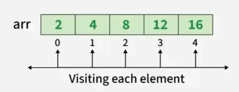
10. Traversal
Traversal means visiting elements one by one.
Index-based traversal
for (int i = 0; i < n; i++) {
    cout << arr[i] << " ";
}
Complexity:
Time: O(n)
Space: O(1)
Range-based loop
for (int x : arr) {
    cout << x << " ";
}
Use this when the index is not required.
Range-based loop by reference
for (int &x : arr) {
    x *= 2;
}
This can modify the original elements.
For read-only access:
for (const int &x : arr) {
    cout << x;
}
11. Insertion and Deletion
The cost depends on where the operation occurs.
Suppose:
10 20 30 40 50
Insert at the end
For a vector:
arr.push_back(60);
Amortized:
O(1)
Insert at the beginning
Existing elements need to shift:
Before:
10 20 30 40

After:
5 10 20 30 40
Complexity:
O(n)
Insert in the middle
Elements after the insertion position generally shift.
Complexity:
O(n)
Delete from the end
arr.pop_back();
Complexity:
O(1)
Delete from the beginning or middle
Elements may need to shift.
Complexity:
O(n)
Key idea: Arrays are excellent for random access but relatively expensive for insertion/deletion away from the end because elements may need to be shifted.
12. Time and Space Complexity
| Operation | Array | Vector |
|---|---|---|
| Access by index | O(1) | O(1) |
| Update by index | O(1) | O(1) |
| Search unsorted | O(n) | O(n) |
| Binary search when sorted | O(log n) | O(log n) |
| Traverse | O(n) | O(n) |
| Insert at beginning | O(n) | O(n) |
| Insert in middle | O(n) | O(n) |
| Insert at end | — | Amortized O(1) |
| Delete from beginning | O(n) | O(n) |
| Delete from middle | O(n) | O(n) |
| Delete from end | — | O(1) |
For n elements:
Storage = O(n)
If an algorithm processes the array using only a constant number of additional variables:
Auxiliary space = O(1)
13. Passing Arrays to Functions
Built-in array
void printArray(int arr[], int n) {
    for (int i = 0; i < n; i++) {
        cout << arr[i] << " ";
    }
}
When a built-in array is passed to a function parameter, it is effectively handled as a pointer to its first element.
Therefore, the size is normally supplied separately:
printArray(arr, n);
The parameter forms:
int arr[]
and:
int* arr
are closely related in a function parameter list.
Vector
For a vector, avoid unnecessary copies:
void solve(const vector<int>& arr) {
    // read-only access
}
14. Pass by Value vs Pass by Reference
Pass by value
void solve(vector<int> arr) {
    ...
}
A copy of the vector is created.
For n elements, copying requires approximately:
Time: O(n)
Extra space: O(n)
Pass by reference
void solve(vector<int>& arr) {
    ...
}
No complete copy is made.
Changes affect the original vector.
Pass by const reference
void solve(const vector<int>& arr) {
    ...
}
This is often preferred when the function only needs to read the vector.
Summary:
vector<int> arr
→ copy

vector<int>& arr
→ reference, modification allowed

const vector<int>& arr
→ reference, read-only
15. Important C++ Array and Vector Operations
size()
arr.size();
Number of elements.
empty()
arr.empty();
Checks whether there are zero elements.
push_back()
arr.push_back(x);
Adds at the end.
pop_back()
arr.pop_back();
Removes the last element.
front() / back()
arr.front();
arr.back();
Access first/last element.
begin() / end()
arr.begin();
arr.end();
Provide iterators representing the beginning and one-past-the-end position.
Common usage:
sort(arr.begin(), arr.end());
reverse()
reverse(arr.begin(), arr.end());
Typical complexity:
O(n)
sort()
sort(arr.begin(), arr.end());
Typical complexity:
O(n log n)
Descending:
sort(arr.rbegin(), arr.rend());
min_element() / max_element()
*min_element(arr.begin(), arr.end());
*max_element(arr.begin(), arr.end());
Typical complexity:
O(n)
These functions return iterators, so dereference them to obtain the value.
accumulate()
Include:
#include <numeric>
Example:
long long sum = accumulate(arr.begin(), arr.end(), 0LL);
Typical complexity:
O(n)
Using 0LL is important when the sum may exceed the range of int.
find()
auto it = find(arr.begin(), arr.end(), x);
Typical complexity:
O(n)
Check:
if (it != arr.end()) {
    // found
}
count()
int frequency = count(arr.begin(), arr.end(), x);
Typical complexity:
O(n)
16. Common Array Problem-Solving Patterns
Array interview problems frequently test whether you can recognize a reusable pattern.
The most important patterns are:
- Linear traversal
- Frequency counting
- Prefix sum
- Two pointers
- Sliding window
- Hashing
- Sorting-based techniques
- Binary search
- Kadane's algorithm
- In-place modification
Recognizing the pattern is usually more valuable than memorizing isolated solutions.
17. Prefix Sum
A prefix sum stores cumulative sums so that range sums can be computed efficiently.
For:
arr = [2, 4, 1, 3, 5]
A prefix array can be:
prefix = [2, 6, 7, 10, 15]
Definition:
prefix[i] = arr[0] + arr[1] + ... + arr[i]
A common implementation:
vector<int> prefix(n);

prefix[0] = arr[0];

for (int i = 1; i < n; i++) {
    prefix[i] = prefix[i - 1] + arr[i];
}
For a range [l, r] with l > 0:
sum(l, r) = prefix[r] - prefix[l - 1]
A cleaner implementation uses a prefix array of size n + 1:
vector<long long> prefix(n + 1, 0);

for (int i = 0; i < n; i++) {
    prefix[i + 1] = prefix[i] + arr[i];
}
Then:
sum(l, r) = prefix[r + 1] - prefix[l]
Complexity
Build prefix: O(n)
Each range query: O(1)
Extra space: O(n)
Prefix sums are especially useful when repeated range-sum queries or cumulative information are involved.
18. Two Pointers
The two-pointer technique uses two indices to process an array efficiently.
A common form is:
left → ← right
Implementation structure:
int left = 0;
int right = n - 1;

while (left < right) {
    // process arr[left] and arr[right]
}
Another form uses two pointers moving in the same direction:
slow →
fast →
Two pointers are particularly useful for:
- sorted arrays
- pair-based processing
- removing duplicates
- partitioning
- reversing
- in-place modification
- merging
A good two-pointer solution can often reduce a nested-loop approach from:
O(n²)
to:
O(n)
Two pointers are a technique, not one fixed algorithm. Pointer movement depends on the problem's invariant.
19. Sliding Window
Sliding window is primarily used for problems involving contiguous subarrays.
The current window is represented by:
[left ........ right]
Instead of recomputing every subarray from scratch, maintain information about the current window while moving its boundaries.
Typical variable structure:
int left = 0;

for (int right = 0; right < n; right++) {

    // include arr[right]

    while (/* window is invalid */) {
        // remove arr[left]
        left++;
    }

    // process current window
}
Common applications include:
- fixed-size window calculations
- longest valid subarray
- shortest valid subarray
- frequency-based windows
- subarray problems with constraints
Many sliding-window algorithms run in:
O(n)
because each pointer moves forward and does not repeatedly move backward.
20. Frequency / Counting
Frequency counting records how many times values occur.
For a small known integer range, use a frequency array.
Conceptually:
Value:      0  1  2  3  4
Frequency:  2  0  3  1  0
C++:
vector<int> freq(maxValue + 1, 0);

for (int x : arr) {
    freq[x]++;
}
Useful when:
- values lie in a manageable range
- occurrence counts are required
- duplicate detection is required
- frequency comparisons are required
Complexity:
Time: O(n)
Space: O(k)
where k is the value range.
For large, negative, or sparse values, a hash map is often more appropriate.
21. Hashing with Arrays and Hash Maps
When values are arbitrary or too large for a frequency array, use hashing.
unordered_map<int, int> freq;

for (int x : arr) {
    freq[x]++;
}
Average lookup/insertion complexity:
O(1)
This can transform many frequency or lookup problems from:
O(n²)
to approximately:
O(n)
with additional space.
Time-space trade-off
Hashing generally provides:
Faster lookup
at the cost of:
Additional memory
This is one of the most common trade-offs in interview problem solving.
22. Sorting-Based Techniques
Sorting can simplify many array problems.
sort(arr.begin(), arr.end());
Typical complexity:
O(n log n)
Sorting makes several properties easier to exploit:
- duplicates become adjacent
- ordering relationships become explicit
- two pointers can often be used
- binary search becomes possible
- some greedy approaches become possible
Sorting may be slower than an optimal O(n) solution, but it can significantly simplify the algorithm.
When modifying the original array is not allowed, consider whether a copy is required.
23. Binary Search on Arrays
Binary search works when the search space has an appropriate ordering or monotonic property.
For a sorted array:
left       mid        right
  ↓         ↓           ↓
[ ... ... ... ... ... ... ]
At each step, roughly half of the remaining search space is discarded.
Complexity:
O(log n)
Basic implementation:
int left = 0;
int right = n - 1;

while (left <= right) {
    int mid = left + (right - left) / 2;

    if (arr[mid] == target) {
        // found
    }
    else if (arr[mid] < target) {
        left = mid + 1;
    }
    else {
        right = mid - 1;
    }
}
Prefer:
left + (right - left) / 2
over:
(left + right) / 2
because the latter can overflow when left and right are large.
Binary search is also used for:
- first occurrence
- last occurrence
- lower bound
- upper bound
- rotated sorted arrays
- binary search on answer
The broader principle is to identify a monotonic decision boundary.
24. Kadane's Algorithm
Kadane's algorithm finds the maximum sum of a contiguous subarray in linear time.
At each position, maintain the best sum of a subarray ending at the current position.
The core decision is:
Extend the current subarray
OR
Start a new subarray at the current element
Implementation:
long long current = arr[0];
long long best = arr[0];

for (int i = 1; i < n; i++) {
    current = max((long long)arr[i], current + arr[i]);
    best = max(best, current);
}
Complexity:
Time: O(n)
Space: O(1)
The key idea is:
Best result ending here
        ↓
Best result overall
This is a classic example of converting a potentially quadratic subarray computation into a linear-time algorithm.
25. In-Place Array Modification
An in-place algorithm modifies the input array while using only a small amount of additional memory.
Example structure:
int left = 0;

for (int right = 0; right < n; right++) {
    if (/* desired condition */) {
        swap(arr[left], arr[right]);
        left++;
    }
}
Common applications:
- moving elements
- partitioning
- removing duplicates
- rearranging values
- reversing
- separating elements based on a condition
Typical auxiliary space:
O(1)
Important distinction:
Input storage ≠ auxiliary space
Modifying the input array does not count as allocating another array.
26. Subarrays vs Subsequences vs Subsets
These terms are important and frequently confused.
Subarray
A subarray contains contiguous elements.
For:
[1, 2, 3]
Examples:
[1]
[2]
[3]
[1,2]
[2,3]
[1,2,3]
But:
[1,3]
is not a subarray because the elements are not contiguous.
Subsequence
A subsequence maintains the original order but does not require contiguity.
From:
[1,2,3]
possible subsequences include:
[1,3]
[1,2]
[2,3]
[1,2,3]
Subset
A subset is a selection of elements without requiring preservation of the original ordering.
Quick distinction
Subarray     → contiguous
Subsequence  → order preserved, not necessarily contiguous
Subset       → selection without requiring order
This distinction determines which algorithmic techniques are appropriate.
27. Common Array Complexity Patterns
Single traversal
for (int i = 0; i < n; i++) {
    ...
}
Usually:
O(n)
Two independent traversals
for (...) { ... }
for (...) { ... }
Overall:
O(n + n) = O(n)
Constants are ignored in Big-O.
Nested loops
for (int i = 0; i < n; i++) {
    for (int j = 0; j < n; j++) {
        ...
    }
}
Usually:
O(n²)
Sorting followed by traversal
sort(arr.begin(), arr.end());

for (...) {
    ...
}
Overall:
O(n log n) + O(n)
= O(n log n)
Hashing plus traversal
Build hash structure → O(n)
Process array        → O(n)

Overall              → O(n)
assuming average O(1) hash operations.
Prefix sum
Build prefix       → O(n)
Each range query   → O(1)
For q range queries:
O(n + q)
Binary search
One search:
O(log n)
q independent searches:
O(q log n)
28. Interview-Relevant C++ Practices
28.1 Prefer vector for dynamic-size problems
vector<int> arr;
or:
vector<int> arr(n);
28.2 Use long long for potentially large sums
long long sum = 0;
With accumulate:
long long sum = accumulate(arr.begin(), arr.end(), 0LL);
Using 0LL ensures the accumulator starts as long long.
28.3 Avoid unnecessary copies
Prefer:
void solve(const vector<int>& arr)
over:
void solve(vector<int> arr)
when only reading is required.
28.4 Use const when data should not change
const vector<int>& arr
makes the read-only intent explicit.
28.5 Be careful with signed and unsigned types
vector::size() returns an unsigned type.
Use consistent types when comparing indices and sizes.
A common simple loop is:
for (size_t i = 0; i < arr.size(); i++) {
    ...
}
28.6 Avoid out-of-bounds access
For an array of size n:
0 ≤ index < n
For:
vector<int> arr(5);
valid indices are:
0, 1, 2, 3, 4
Accessing:
arr[5]
is out of bounds.
28.7 [] vs .at()
arr[i]
provides direct access without bounds checking.
arr.at(i)
performs bounds checking and can throw std::out_of_range.
In DSA solutions, [] is common when the index is known to be valid.
28.8 Understand iterators
For:
vector<int> arr = {1, 2, 3, 4};
arr.begin()
represents the first element.
arr.end()
represents the position one past the last element.
Therefore:
sort(arr.begin(), arr.end());
sorts the entire vector.
end() must not be dereferenced.
29. Array Theory Quick Revision
Core Definition
Array = linear collection of same-type elements stored contiguously.
Core Properties
Contiguous memory
Zero-based indexing
Random access
Fixed size for built-in arrays
Dynamic size with vector
Core Complexity
Access by index       O(1)
Update by index       O(1)
Traversal             O(n)
Linear search         O(n)
Binary search         O(log n) when applicable
Insert beginning      O(n)
Insert middle         O(n)
Delete beginning      O(n)
Delete middle         O(n)
Vector push_back      Amortized O(1)
Vector pop_back       O(1)
Important C++ Container
vector<int> arr;
Important methods:
size()
empty()
push_back()
pop_back()
front()
back()
begin()
end()
reserve()
resize()
Important algorithms:
sort()
reverse()
find()
count()
min_element()
max_element()
accumulate()
Most Important Patterns
Linear Traversal
Frequency Counting
Prefix Sum
Two Pointers
Sliding Window
Hashing
Sorting
Binary Search
Kadane's Algorithm
In-Place Modification
Most Important Distinctions
Array vs Vector
size vs capacity
reserve vs resize
value vs reference
subarray vs subsequence vs subset
two pointers vs sliding window
frequency array vs hash map
in-place vs extra-space solution
Final Takeaway
The purpose of this theory is to make the following progression natural:
Understand Arrays
       ↓
Understand Complexity
       ↓
Master C++ vector
       ↓
Understand Traversal
       ↓
Recognize Patterns
       ↓
Prefix Sum
       ↓
Two Pointers
       ↓
Sliding Window
       ↓
Hashing / Frequency
       ↓
Sorting
       ↓
Binary Search
       ↓
Kadane's Algorithm
       ↓
In-Place Techniques
       ↓
Problem Practice
The next stage should focus on high-frequency array interview problems, grouped by these patterns rather than treated as unrelated questions.
#Pattern 01: Linear Traversal#
| 1 | #include <iostream> |
| 2 | using namespace std; |
| 3 | |
| 4 | int main() { |
| 5 | int arr[] = {10, 20, 30, 40, 50}; |
| 6 | int n = 5; |
| 7 | |
| 8 | for (int i = 0; i < n; i++) { |
| 9 | cout << arr[i] << " "; |
| 10 | } |
| 11 | |
| 12 | return 0; |
| 13 | } |
#Pattern 02: Frequency Counting#
| 1 | #include <iostream> |
| 2 | #include <vector> |
| 3 | using namespace std; |
| 4 | |
| 5 | int main() { |
| 6 | int arr[] = {2, 3, 2, 5, 3, 2}; |
| 7 | int n = 6; |
| 8 | |
| 9 | vector<int> freq(6, 0); |
| 10 | |
| 11 | // Count frequency |
| 12 | for (int i = 0; i < n; i++) { |
| 13 | freq[arr[i]]++; |
| 14 | } |
| 15 | |
| 16 | // Print frequency |
| 17 | for (int i = 0; i < freq.size(); i++) { |
| 18 | if (freq[i] > 0) { |
| 19 | cout << i << " -> " << freq[i] << endl; |
| 20 | } |
| 21 | } |
| 22 | |
| 23 | return 0; |
| 24 | } |
#Pattern 03: Prefix Sum#
| 1 | #include <iostream> |
| 2 | #include <vector> |
| 3 | using namespace std; |
| 4 | |
| 5 | int main() { |
| 6 | int arr[] = {2, 4, 1, 3, 5}; |
| 7 | int n = 5; |
| 8 | |
| 9 | vector<int> prefix(n); |
| 10 | |
| 11 | prefix[0] = arr[0]; |
| 12 | |
| 13 | for (int i = 1; i < n; i++) { |
| 14 | prefix[i] = prefix[i - 1] + arr[i]; |
| 15 | } |
| 16 | |
| 17 | // Print prefix sum array |
| 18 | for (int i = 0; i < n; i++) { |
| 19 | cout << prefix[i] << " "; |
| 20 | } |
| 21 | |
| 22 | return 0; |
| 23 | } |
#Pattern 04: Two Pointers#
| 1 | #include <iostream> |
| 2 | using namespace std; |
| 3 | |
| 4 | int main() { |
| 5 | int arr[] = {1, 2, 3, 4, 6, 8}; |
| 6 | int n = 6; |
| 7 | int target = 10; |
| 8 | |
| 9 | int left = 0; |
| 10 | int right = n - 1; |
| 11 | |
| 12 | while (left < right) { |
| 13 | int sum = arr[left] + arr[right]; |
| 14 | |
| 15 | if (sum == target) { |
| 16 | cout << "Pair found: " |
| 17 | << arr[left] << " + " |
| 18 | << arr[right] << " = " |
| 19 | << target; |
| 20 | return 0; |
| 21 | } |
| 22 | else if (sum < target) { |
| 23 | left++; |
| 24 | } |
| 25 | else { |
| 26 | right--; |
| 27 | } |
| 28 | } |
| 29 | |
| 30 | cout << "Pair not found"; |
| 31 | |
| 32 | return 0; |
| 33 | } |
#Pattern 05: Sliding Window#
| 1 | #include <iostream> |
| 2 | using namespace std; |
| 3 | |
| 4 | int main() { |
| 5 | int arr[] = {2, 1, 5, 1, 3, 2}; |
| 6 | int n = 6; |
| 7 | int k = 3; |
| 8 | |
| 9 | int windowSum = 0; |
| 10 | |
| 11 | // First window |
| 12 | for (int i = 0; i < k; i++) { |
| 13 | windowSum += arr[i]; |
| 14 | } |
| 15 | |
| 16 | int maxSum = windowSum; |
| 17 | |
| 18 | // Slide the window |
| 19 | for (int i = k; i < n; i++) { |
| 20 | windowSum += arr[i]; // Add new element |
| 21 | windowSum -= arr[i - k]; // Remove old element |
| 22 | |
| 23 | maxSum = max(maxSum, windowSum); |
| 24 | } |
| 25 | |
| 26 | cout << "Maximum sum: " << maxSum; |
| 27 | |
| 28 | return 0; |
| 29 | } |
#Pattern 06: Hashing#
| 1 | #include <iostream> |
| 2 | #include <unordered_map> |
| 3 | using namespace std; |
| 4 | |
| 5 | int main() { |
| 6 | int arr[] = {2, 3, 2, 5, 3, 2}; |
| 7 | int n = 6; |
| 8 | |
| 9 | unordered_map<int, int> freq; |
| 10 | |
| 11 | for (int i = 0; i < n; i++) { |
| 12 | freq[arr[i]]++; |
| 13 | } |
| 14 | |
| 15 | for (auto it : freq) { |
| 16 | cout << it.first << " -> " << it.second << endl; |
| 17 | } |
| 18 | |
| 19 | return 0; |
| 20 | } |
#Pattern 07: Sorting#
| 1 | #include <iostream> |
| 2 | #include <algorithm> |
| 3 | using namespace std; |
| 4 | |
| 5 | int main() { |
| 6 | int arr[] = {5, 2, 8, 1, 3}; |
| 7 | int n = 5; |
| 8 | |
| 9 | sort(arr, arr + n); |
| 10 | |
| 11 | for (int i = 0; i < n; i++) { |
| 12 | cout << arr[i] << " "; |
| 13 | } |
| 14 | |
| 15 | return 0; |
| 16 | } |
#Pattern 08: Binary Search#
| 1 | #include <iostream> |
| 2 | using namespace std; |
| 3 | |
| 4 | int main() { |
| 5 | int arr[] = {1, 3, 5, 7, 9, 11, 13}; |
| 6 | int n = 7; |
| 7 | int target = 9; |
| 8 | |
| 9 | int left = 0; |
| 10 | int right = n - 1; |
| 11 | |
| 12 | while (left <= right) { |
| 13 | int mid = left + (right - left) / 2; |
| 14 | |
| 15 | if (arr[mid] == target) { |
| 16 | cout << "Element found at index " << mid; |
| 17 | return 0; |
| 18 | } |
| 19 | else if (arr[mid] < target) { |
| 20 | left = mid + 1; |
| 21 | } |
| 22 | else { |
| 23 | right = mid - 1; |
| 24 | } |
| 25 | } |
| 26 | |
| 27 | cout << "Element not found"; |
| 28 | |
| 29 | return 0; |
| 30 | } |
#Pattern 09: Kadane's Algorithm#
| 1 | #include <iostream> |
| 2 | #include <algorithm> |
| 3 | using namespace std; |
| 4 | |
| 5 | int main() { |
| 6 | int arr[] = {-2, 1, -3, 4, -1, 2, 1, -5, 4}; |
| 7 | int n = 9; |
| 8 | |
| 9 | int currentSum = arr[0]; |
| 10 | int maxSum = arr[0]; |
| 11 | |
| 12 | for (int i = 1; i < n; i++) { |
| 13 | currentSum = max(arr[i], currentSum + arr[i]); |
| 14 | maxSum = max(maxSum, currentSum); |
| 15 | } |
| 16 | |
| 17 | cout << "Maximum subarray sum: " << maxSum; |
| 18 | |
| 19 | return 0; |
| 20 | } |
#Pattern 10: In-Place Modification#
| 1 | #include <iostream> |
| 2 | using namespace std; |
| 3 | |
| 4 | int main() { |
| 5 | int arr[] = {0, 1, 0, 3, 12}; |
| 6 | int n = 5; |
| 7 | |
| 8 | int write = 0; |
| 9 | |
| 10 | // Move non-zero elements forward |
| 11 | for (int read = 0; read < n; read++) { |
| 12 | if (arr[read] != 0) { |
| 13 | arr[write] = arr[read]; |
| 14 | write++; |
| 15 | } |
| 16 | } |
| 17 | |
| 18 | // Fill remaining positions with zero |
| 19 | while (write < n) { |
| 20 | arr[write] = 0; |
| 21 | write++; |
| 22 | } |
| 23 | |
| 24 | for (int i = 0; i < n; i++) { |
| 25 | cout << arr[i] << " "; |
| 26 | } |
| 27 | |
| 28 | return 0; |
| 29 | } |
#Code Output#
#Leetcode Problems#
20 Essential Array Problems — LeetCode Interview Practice
A curated set of 20 high-value Array problems for interview preparation. These problems cover the most important array-solving patterns beyond the core theory: two pointers, sorting, hashing, prefix sum, sliding window, greedy techniques, in-place modification, matrix manipulation, interval processing, cyclic techniques, and advanced array patterns. The goal is not to learn new theory from each problem, but to strengthen pattern recognition and problem-solving through LeetCode practice. These problems complement the previously covered Array concepts and provide practice across easy, medium, and advanced interview-level scenarios.
- •#15 — 3Sum → Sorting + Two Pointers
- •#18 — 4Sum → Sorting + Two Pointers
- •#31 — Next Permutation → Array Manipulation
- •#41 — First Missing Positive → In-Place Hashing
- •#48 — Rotate Image → Matrix + In-Place
- •#49 — Group Anagrams → Hashing + Sorting
- •#54 — Spiral Matrix → Matrix Traversal
- •#56 — Merge Intervals → Sorting + Greedy
- •#57 — Insert Interval → Interval Processing
- •#73 — Set Matrix Zeroes → Matrix + In-Place
- •#75 — Sort Colors → Dutch National Flag + Two Pointers
- •#80 — Remove Duplicates from Sorted Array II → Two Pointers
- •#128 — Longest Consecutive Sequence → Hashing
- •#152 — Maximum Product Subarray → Dynamic Programming
- •#189 — Rotate Array → Reverse / In-Place
- •#209 — Minimum Size Subarray Sum → Sliding Window
- •#229 — Majority Element II → Boyer-Moore Voting
- •#287 — Find the Duplicate Number → Cycle Detection
- •#380 — Insert Delete GetRandom O(1) → Hashing + Array
- •#560 — Subarray Sum Equals K → Prefix Sum + Hashing
Why Arrays Matter in Real-World Software Engineering
Arrays are one of the fundamental ways software stores and processes collections of data. In real applications, engineers use array-like structures to store sensor readings, user records, product lists, pixels in images, logs, API responses, and numerical data. For example, an IoT system may store temperature readings in an array, an image-processing system represents pixels as arrays, and a backend may process a list of products or users using array-based data structures. We learn arrays because they build the foundation for more advanced data structures and algorithms such as strings, matrices, hashing, stacks, queues, heaps, and many optimization techniques.
- •• Used for storing and processing collections of data
- •• Common in IoT, image processing, databases, APIs, analytics, and backend systems
- •• Provides fast O(1) index-based access
- •• Forms the foundation for many DSA patterns
- •• Understanding arrays improves problem-solving and algorithmic thinking
- •• Future scope: matrices, strings, hashing, dynamic programming, searching, sorting, and advanced data structures
- •• Interview takeaway: Always ask — “Is the data ordered, contiguous, and can I exploit indices or patterns?”